Demonstration notebook for qp_flexzboost
This notebook showcases the general functionality of provided by qp and qp_flexzboost.
[1]:
import os
import qp
import qp_flexzboost
from flexcode.basis_functions import BasisCoefs
import matplotlib.pyplot as plt
import numpy as np
First, we’ll retrieve some real world example coefficients (i.e. weights) and define a basis_coefficients object.
[2]:
qp_flexzboost.FlexzboostGen.make_test_data()
coefs = qp_flexzboost.FlexzboostGen.test_data['weights']
[3]:
# Demonstrate the creation of a `FlexCode.BasisCoefs` object.
basis_coefficients = BasisCoefs(coefs,
                                basis_system='cosine',
                                z_min=0.0,
                                z_max=3.0,
                                bump_threshold=0.1,
                                sharpen_alpha=1.2)
[4]:
# Just an example to show how the basis_coefficient.evaluate method works.
# Notice that it doesn't take a simple 1D x array.
x = np.linspace(0,3,100)
print(x.shape)
x_vals = x.reshape(-1,1)
print(x_vals.shape)
y_vals = basis_coefficients.evaluate(x_vals)

# I expected this to work, namely passing an array with size (10, 100) to the evaluate method.
# The goal is to show that evaluate can handle different x values per PDF - even though
# here it would just be repeating the same x values 10 times. There might be a bug
# in the Flexcode code around basis_functions.py:44

# xx_vals = np.tile(x, [10, 1])
# print(xx_vals.shape)
# yy_vals = basis_coefficients.evaluate(xx_vals)
(100,)
(100, 1)
There are two ways to instantiate a qp.Ensemble that contains qp_flexzboost distributions. The first way is to use qp_flexzboost.flexzboost_create_from_basis_coef_object. It’s more user friendly and is unpacked on users behalf, into the second way - using qp_flexzboost.flexzboost. Either approach will result in identical qp.Ensemble objects for identical inputs.
[5]:
# The more user friendly technique for instantiating a qp.Ensemble. It requires fewer input parameters for the user to provide. Under the hood, it will be converted to the second technique shown next.
fzb = qp.Ensemble(qp_flexzboost.flexzboost_create_from_basis_coef_object, data=dict(weights=coefs, basis_coefficients_object=basis_coefficients))

# The second technique, which requires multiple parameters to be listed explicitly is easier for `qp` machinery to work with.
fzb2 = qp.Ensemble(qp_flexzboost.flexzboost,
                   data=dict(weights=coefs, basis_system_enum_value=1, z_min=0.0, z_max=3.0, bump_threshold=0.1, sharpen_alpha=1.2))
To drive the point home, we demonstrate that the output PDF values are the same regardless of whether the ensemble is constructed with a BasisCoef or with the individual properties of the BasisCoef. If the values in the two Ensembles are the same, we expect an output value of 0.0.
[6]:
pdf_id = 6
x = np.linspace(0,3,100)

print(np.sum(fzb[pdf_id].pdf(x) - fzb2[pdf_id].pdf(x)))
0.0
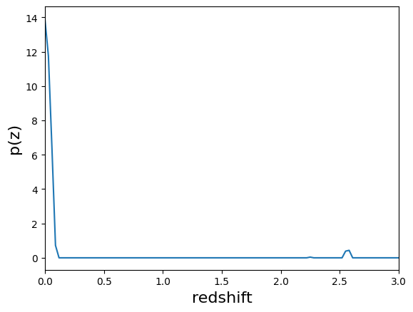
Simple demonstraition of the built in PDF plotting.
[7]:
qp.plotting.plot_native(fzb[pdf_id], xlim=[0,3])
[7]:
(<Figure size 640x480 with 1 Axes>, <Axes: xlabel='redshift', ylabel='p(z)'>)
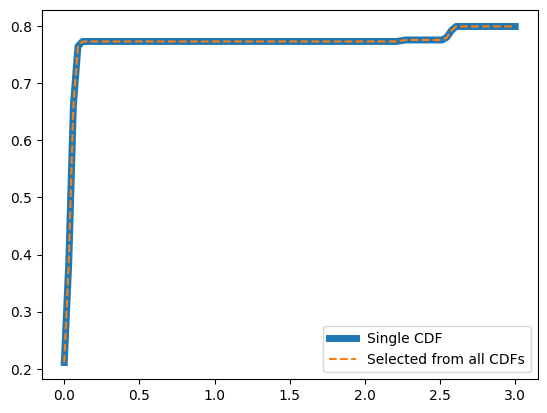
Similarly a demonstration of plotting CDFs. The first selects a particular distribution from the Ensemble and retrieves the CDF. The second approach calculates the CDFs of all the distributions before selected one to plot. Here we’ve selected the same distribution to show that both methods produce the same results.
[8]:
# Demonstrate that CDFs work as expected

# A single CDF from the ensemble
plt.plot(x, np.squeeze(fzb[pdf_id].cdf(x)), linewidth=5, label='Single CDF')

# Calculate the CDF for all distributions in the ensemble, and then select one
cdfs = fzb.cdf(x)
cdfs[pdf_id]
plt.plot(x, cdfs[pdf_id], linestyle='--', label='Selected from all CDFs' )
plt.legend()
[8]:
<matplotlib.legend.Legend at 0x7f0e6223ac20>
The following demonstrates exactly what would be saved to disk for this Ensemble.
[9]:
# Demonstrate that building tables for output to disk works as expected.
tabs = fzb.build_tables()
print(tabs.keys())
print("Meta Data")
print(tabs['meta'])
print()
print("Object Data")
print(tabs['data'])
dict_keys(['meta', 'data'])
Meta Data
{'pdf_name': array([b'flexzboost'], dtype='|S10'), 'pdf_version': array([0]), 'bump_threshold': array([0.1]), 'sharpen_alpha': array([1.2]), 'basis_system_enum_value': array([1]), 'z_min': array([0.]), 'z_max': array([3.])}

Object Data
{'weights': array([[ 0.99999994,  1.4135911 ,  1.3578598 ,  1.3848811 ,  1.1752609 ,
         1.2507105 ,  0.96589327,  1.2579455 ,  1.1328095 ,  0.9338199 ,
         1.3668357 ,  0.63097477,  0.19285281, -0.08388292,  0.05250954,
        -0.5464654 , -0.3771514 , -0.3948611 ,  0.13923086, -0.20495746,
        -0.58977485, -0.6391217 , -0.46343976, -0.5011808 , -0.01433064,
         0.278602  ,  0.5333237 ,  0.826034  ,  0.06464108,  0.9108775 ,
         0.6811071 ,  0.69773537, -0.11616451, -0.09364327,  0.63583785],
       [ 0.99999994,  1.3128049 ,  1.4268231 ,  1.3475941 ,  1.3009573 ,
         1.1934606 ,  1.1979764 ,  1.4587557 ,  1.0695385 ,  1.0334687 ,
         0.85049105,  0.6772867 ,  0.8599958 ,  0.7309471 ,  0.30866015,
         0.10747848,  0.1454999 ,  0.4564285 ,  0.83178055,  0.9569013 ,
         0.2805161 ,  0.35286552,  0.58561605,  0.42757383,  0.40403488,
        -0.5502439 ,  0.56439424,  0.21782365,  0.80970615,  0.6189492 ,
         0.9209366 ,  0.01046925, -0.66917616,  0.0304801 , -0.34911576],
       [ 0.99999994,  1.3046595 ,  1.3946912 ,  1.3725231 ,  1.3279371 ,
         1.1379944 ,  1.1232849 ,  1.3168706 ,  1.1987064 ,  0.846475  ,
         1.2190387 ,  1.0319941 ,  0.8385918 ,  0.72406054,  0.4407519 ,
         1.0522529 ,  0.5317534 ,  0.82531404,  0.6055132 ,  0.42970878,
         0.5682917 ,  0.42682788, -0.04017492,  0.32071114,  0.7407263 ,
         0.20112868,  0.28844437, -0.01918357,  0.16105941, -0.9992142 ,
        -0.481242  , -0.3728989 , -0.39303133, -0.556516  , -0.23944338],
       [ 0.99999994,  1.405193  ,  1.3786027 ,  1.3832911 ,  1.3786896 ,
         1.1868116 ,  1.1039548 ,  1.056342  ,  1.253356  ,  1.275163  ,
         1.5149004 ,  0.7893624 ,  1.1212736 ,  0.7551946 ,  0.1665442 ,
         0.31703034, -0.3789813 ,  0.40208268, -0.00154649, -0.22578228,
        -0.754486  ,  0.09544089, -0.7406911 , -1.5187913 , -1.0511639 ,
        -0.9208054 , -0.52502257, -0.79425025,  0.11232897, -0.5873992 ,
        -0.00291769, -1.2490546 ,  0.18622968, -0.4166289 , -0.16232875],
       [ 0.99999994,  1.32483   ,  1.2688403 ,  0.8508245 ,  1.4554728 ,
         1.2448467 ,  0.852745  ,  0.8741474 ,  1.0841464 ,  0.7697048 ,
         1.1911153 ,  0.51762104,  1.1319616 ,  1.3946458 ,  0.82583827,
         0.21972111, -0.16429716, -0.08124515,  0.0241714 , -0.07269649,
         0.04703106,  0.4027557 , -1.1216148 , -0.8540991 , -0.7413664 ,
        -0.35533333, -0.47791988, -0.39957288,  0.1695733 , -0.46430817,
        -0.07995562, -1.0972134 , -0.61197704, -1.1898835 , -0.75323683],
       [ 0.99999994,  1.4217128 ,  1.4090639 ,  1.3527906 ,  1.2788762 ,
         1.0873253 ,  1.0570015 ,  1.1381446 ,  0.73468673,  0.4902846 ,
         0.11609144, -0.43022275, -0.33087614,  0.3467521 ,  0.14698188,
        -0.79639876, -0.7686687 , -1.0865113 , -1.0686133 , -1.0762304 ,
        -0.9354039 , -0.79879427, -0.24612567,  0.01798107, -0.2094559 ,
         0.24940334,  0.12473647,  0.10005763,  0.23591852,  0.33464774,
         0.64543843,  0.24140209,  0.8614289 ,  0.10955815, -0.09307325],
       [ 0.99999994, -0.60270864,  0.3777081 ,  1.0040071 ,  0.5319608 ,
         1.1732529 ,  0.21736576,  1.0385551 ,  0.85155064,  0.8202011 ,
         0.7389486 ,  0.69682765,  0.1181715 ,  0.13482217,  0.7518282 ,
         0.8588988 ,  0.2753361 ,  0.10158755,  0.53366745,  0.5017293 ,
         0.22024332,  0.8345108 ,  0.3317933 ,  0.5323848 ,  0.741613  ,
         0.215265  ,  0.3551328 ,  0.44486073,  0.07836582,  0.00493836,
         0.583493  ,  0.23795973,  0.10176475, -0.08585434, -0.47022513],
       [ 0.99999994,  1.403194  ,  1.3613293 ,  1.2763977 ,  1.0978196 ,
         1.0092797 ,  0.87263453,  0.63493866,  0.3737632 , -0.02474818,
         0.12842114, -0.31487998, -0.18406785, -0.42329717, -0.8819336 ,
        -0.887077  , -0.913117  , -1.1706294 , -1.1096691 , -0.46700883,
        -0.7291215 , -0.20483486, -0.57670075, -0.5173913 ,  0.17409407,
        -0.34383368,  0.11131766,  0.29361913,  0.22329482,  0.4090505 ,
         0.50041765,  1.040421  ,  0.7399761 ,  1.3841617 ,  1.0754173 ],
       [ 0.99999994,  0.5964216 ,  0.46396077,  1.2265164 ,  1.0870706 ,
         1.1584536 ,  0.89783925,  0.7338294 ,  0.7884262 ,  0.41392878,
         0.27348533,  0.60299355, -0.09960458,  0.6036693 , -0.01055456,
         0.32332683, -0.63185304,  0.11284541, -0.30345288, -0.72329307,
        -0.2737094 ,  0.03923929, -0.26043436, -0.5889996 ,  0.09375673,
        -0.27470988, -0.03649841,  0.1934136 , -0.41822934, -0.38939086,
        -0.2009153 , -0.1781136 ,  0.81968015,  0.5067288 ,  0.54687506],
       [ 0.99999994,  1.3862562 ,  1.3533832 ,  1.3327965 ,  1.3019644 ,
         1.3206618 ,  1.3192286 ,  0.97659546,  1.0163264 ,  1.0176893 ,
         0.57915735,  0.7081749 ,  0.7332014 ,  0.5191775 ,  0.07479973,
         0.13503157,  0.25693908, -0.13746639, -0.06378681, -0.2937861 ,
        -0.2938108 ,  0.03345898, -0.45815086, -0.45607626, -0.91071063,
        -0.7797466 , -0.5807737 , -0.34890455, -0.60276383, -0.49033943,
        -0.81330174, -0.4416928 , -0.88592136, -0.7070263 ,  0.02908602]])}
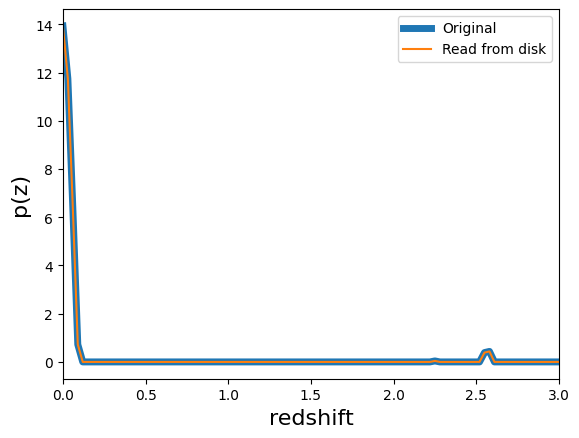
The following demonstrates that the ensemble can be written to disk, and read back in with no loss of information.
[10]:
output_fits = "test_output.fits"
output_hdf5 = "test_output.hdf5"

# delete the files if they already exist
try:
    os.unlink(output_hdf5)
    os.unlink(output_fits)
except FileNotFoundError:
    pass

# write out the files
fzb.write_to(output_hdf5)
print(".hdf5 file size is:", os.path.getsize(output_hdf5), "bytes")
fzb.write_to(output_fits)
print(".fits file size is:", os.path.getsize(output_fits), "bytes")

# read the files back in
fzb_reread_hdf5 = qp.read(output_hdf5)
fzb_reread_fits = qp.read(output_fits)

# Show that the number of PDFs is the same after reading in the files
print("Initial number of pdfs:", fzb.npdf)
print("Recovered number of pdfs, hdf5:", fzb_reread_hdf5.npdf)
print("Recovered number of pdfs, fits:", fzb_reread_fits.npdf)

# Show that the plots for a given PDF are the same
_, ax = qp.plotting.plot_native(fzb_reread_hdf5[pdf_id], xlim=[0,3], linewidth=5, label='Original')
qp.plotting.plot_native(fzb_reread_fits[pdf_id], axes=ax, label='Read from disk')
plt.legend()

# Show that nothing has been lost in the file type storage methods
pdf_hdf5 = fzb_reread_hdf5[pdf_id].pdf(x_vals)
pdf_fits = fzb_reread_fits[pdf_id].pdf(x_vals)
print("Total difference in file storage types:", sum((pdf_fits-pdf_hdf5)**2))

# show that all the parameters to define the BasisCoef object have been recovered
print("Initial bump_threshold:", fzb.dist.basis_coefficients.bump_threshold)
print("Recovered fits bump_threshold:", fzb_reread_fits.dist.basis_coefficients.bump_threshold)
print("Recovered hdf5 bump_threshold:", fzb_reread_hdf5.dist.basis_coefficients.bump_threshold)

# delete the output files that were written
try:
    os.unlink(output_hdf5)
    os.unlink(output_fits)
except FileNotFoundError:
    pass
.hdf5 file size is: 11136 bytes
.fits file size is: 14400 bytes
Initial number of pdfs: 10
Recovered number of pdfs, hdf5: 10
Recovered number of pdfs, fits: 10
Total difference in file storage types: [0.]
Initial bump_threshold: 0.1
Recovered fits bump_threshold: 0.1
Recovered hdf5 bump_threshold: 0.1
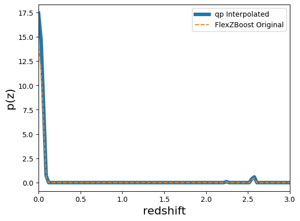
Here we show that the qp_flexzboost parameterization can be converted to other native qp representations. The conversion will be lossy, with the impact to the fidelity defined primarily by the x grid used in the conversion.
[11]:
# Demonstrate that the Flexzboost parameterization of the data can be converted
# to other representations. For instance here, an interpolated grid.
ens_interp = fzb.convert_to(qp.interp_gen, xvals=np.linspace(0,3,100))

# Plot interpolated PDF (thick line)
qp.plotting.plot_native(ens_interp[pdf_id], xlim=[0,3], linewidth=5, label='qp Interpolated')

# Plot original, Flexzboost PDF (dashed line)
plt.plot(x, np.squeeze(fzb[pdf_id].pdf(x)), linestyle='--', label='FlexZBoost Original')
plt.legend()
[11]:
<matplotlib.legend.Legend at 0x7f0e5ffad4b0>
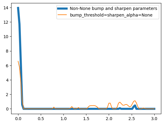
Here we demonstrate that the bump threshold and sharpening alpha parameters can be changed dynamically without rerunning the model.
[12]:
# Set the bump threshold and sharpening parameters to the original values
fzb.dist.bump_threshold = 0.1
fzb.dist.sharpen_alpha = 1.2

# Plot original, Flexzboost PDF (dashed line)
plt.plot(x, np.squeeze(fzb[pdf_id].pdf(x)), linewidth=5, label='Non-None bump and sharpen parameters')

# remove the bump threshold and sharpening parameters
fzb.dist.bump_threshold = None
fzb.dist.sharpen_alpha = None

plt.plot(x, np.squeeze(fzb[pdf_id].pdf(x)), label='bump_threshold=sharpen_alpha=None')
plt.legend()
[12]:
<matplotlib.legend.Legend at 0x7f0e5fbe9330>