CDF Exploration notebook for `qp_flexzboost`

This notebook demonstrates that as the x grid resolution is increased, the CDF approaches 1. It also shows that the CDF approaches 1 for bump_threshold and sharpen_alpha values of None and non-None.

[1]:

import qp
import qp_flexzboost
import numpy as np
from flexcode.basis_functions import BasisCoefs
import matplotlib.pyplot as plt

Matplotlib is building the font cache; this may take a moment.

[2]:

# Retrieve some real world example coefficients (i.e. weights) that are used for testing.
qp_flexzboost.FlexzboostGen.make_test_data()
coefs = qp_flexzboost.FlexzboostGen.test_data['weights']

[3]:

# Here we defined a BasisCoefs object with bump_threshold=sharpen_threshold=None. i.e. no bump removal or peak sharpening
basis_coefficients = BasisCoefs(coefs,
                                basis_system='cosine',
                                z_min=0.0,
                                z_max=3.0,
                                bump_threshold=None,
                                sharpen_alpha=None)

Next we’ll build a qp.Ensemble from the test data and basis_coefficients object defined above.

[4]:

fzb = qp.Ensemble(qp_flexzboost.flexzboost_create_from_basis_coef_object,
                  data=dict(weights=coefs, basis_coefficients_object=basis_coefficients))

[5]:

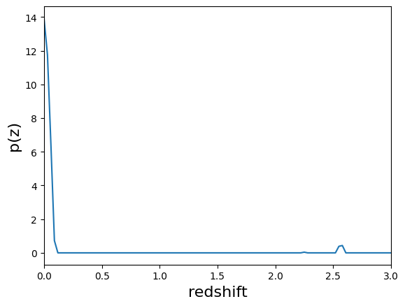
# Here we specify a particular PDF id, and define a fine and course x grid.
pdf_id = 6
x_course = np.linspace(0,3,100)
x_fine = np.linspace(0,3,30000)

[6]:

# Example PDF with no bump removal or peak sharpening
qp.plotting.plot_native(fzb[pdf_id], xlim=[0,3])

[6]:

(<Figure size 640x480 with 1 Axes>, <Axes: xlabel='redshift', ylabel='p(z)'>)

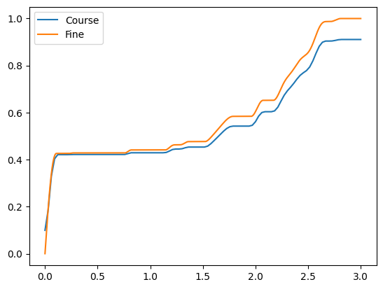
../_images/notebooks_cdf_demonstration_8_1.png

Next we’ll plot the numerical CDF of the same distribution using the course and fine x grids. Note that finer grid approaches 1 while, the course grid just exceeds 0.91.

[7]:

# Demonstrate that CDFs approach 1 as grid resolution increases
cdf_course = fzb[pdf_id].cdf(x_course)
cdf_fine = fzb[pdf_id].cdf(x_fine)
plt.plot(x_course, np.squeeze(cdf_course), label='Course')
plt.plot(x_fine, np.squeeze(cdf_fine), label='Fine')
plt.legend()

print('Max CDF value, course grid:', np.max(cdf_course))
print('Max CDF value, fine grid:', np.max(cdf_fine))

Max CDF value, course grid: 0.9105627564772705
Max CDF value, fine grid: 0.9997021611016463

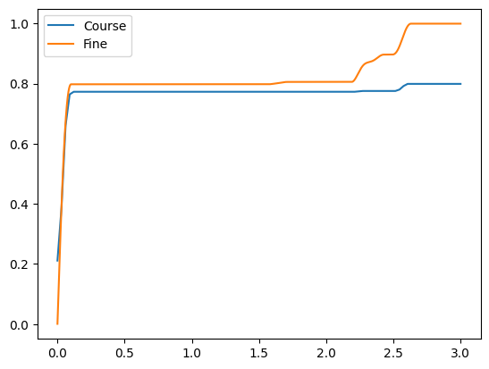
../_images/notebooks_cdf_demonstration_10_1.png

In this cell, we show that we can dynamically change the bump threshold and sharpening without having to rerun the model.

[8]:

fzb.dist.bump_threshold = 0.1
fzb.dist.sharpen_alpha = 1.2

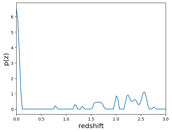
Compare this plot to the PDF plotted in cell 6. It is the same PDF< but with bump thresholds and peak sharpening applied.

[9]:

qp.plotting.plot_native(fzb[pdf_id], xlim=[0,3])

[9]:

(<Figure size 640x480 with 1 Axes>, <Axes: xlabel='redshift', ylabel='p(z)'>)

../_images/notebooks_cdf_demonstration_14_1.png

Again, even with bump thresholding and peak sharpening, the numerical CDF will approach 1 for fine x grids. Note though, that the difference between the course and fine grids is more pronounced when including non-None bump threshold and sharpen alpha values. Here the fine grid approaches 1, while the course grid approaches 0.8. Recall in the previous example without bump threshold or peak sharpening, the course grid just exceeds 0.91.

[10]:

cdf_course = fzb[pdf_id].cdf(x_course)
cdf_fine = fzb[pdf_id].cdf(x_fine)
plt.plot(x_course, np.squeeze(cdf_course), label='Course')
plt.plot(x_fine, np.squeeze(cdf_fine), label='Fine')
plt.legend()

print('Max CDF value, course grid:', np.max(cdf_course))
print('Max CDF value, fine grid:', np.max(cdf_fine))

Max CDF value, course grid: 0.7990015109760497
Max CDF value, fine grid: 0.9993478823556085

../_images/notebooks_cdf_demonstration_16_1.png

CDF Exploration notebook for qp_flexzboost

CDF Exploration notebook for `qp_flexzboost`